15 Human geography lab 5

Load all necessary packages

pacman::p_load(tidyverse, rnaturalearth, sf, DT)

15.1 World and continents with `sf`

The above command will install all dependencies required to reproduce the entire lecture

Use the package sf
We will use the world dataset provided by spData, to show what sf objects are and how they work. world is an ‘sf data frame’ containing spatial and attribute columns, the names of which are returned by the function names() (the last column in this example contains the geographic information):

world <- ne_countries(scale = "small", returnclass = "sf")
class(world)

[1] "sf"         "data.frame"

names(world)

  [1] "featurecla" "scalerank"  "labelrank"  "sovereignt" "sov_a3"    
  [6] "adm0_dif"   "level"      "type"       "tlc"        "admin"     
 [11] "adm0_a3"    "geou_dif"   "geounit"    "gu_a3"      "su_dif"    
 [16] "subunit"    "su_a3"      "brk_diff"   "name"       "name_long" 
 [21] "brk_a3"     "brk_name"   "brk_group"  "abbrev"     "postal"    
 [26] "formal_en"  "formal_fr"  "name_ciawf" "note_adm0"  "note_brk"  
 [31] "name_sort"  "name_alt"   "mapcolor7"  "mapcolor8"  "mapcolor9" 
 [36] "mapcolor13" "pop_est"    "pop_rank"   "pop_year"   "gdp_md"    
 [41] "gdp_year"   "economy"    "income_grp" "fips_10"    "iso_a2"    
 [46] "iso_a2_eh"  "iso_a3"     "iso_a3_eh"  "iso_n3"     "iso_n3_eh" 
 [51] "un_a3"      "wb_a2"      "wb_a3"      "woe_id"     "woe_id_eh" 
 [56] "woe_note"   "adm0_iso"   "adm0_diff"  "adm0_tlc"   "adm0_a3_us"
 [61] "adm0_a3_fr" "adm0_a3_ru" "adm0_a3_es" "adm0_a3_cn" "adm0_a3_tw"
 [66] "adm0_a3_in" "adm0_a3_np" "adm0_a3_pk" "adm0_a3_de" "adm0_a3_gb"
 [71] "adm0_a3_br" "adm0_a3_il" "adm0_a3_ps" "adm0_a3_sa" "adm0_a3_eg"
 [76] "adm0_a3_ma" "adm0_a3_pt" "adm0_a3_ar" "adm0_a3_jp" "adm0_a3_ko"
 [81] "adm0_a3_vn" "adm0_a3_tr" "adm0_a3_id" "adm0_a3_pl" "adm0_a3_gr"
 [86] "adm0_a3_it" "adm0_a3_nl" "adm0_a3_se" "adm0_a3_bd" "adm0_a3_ua"
 [91] "adm0_a3_un" "adm0_a3_wb" "continent"  "region_un"  "subregion" 
 [96] "region_wb"  "name_len"   "long_len"   "abbrev_len" "tiny"      
[101] "homepart"   "min_zoom"   "min_label"  "max_label"  "label_x"   
[106] "label_y"    "ne_id"      "wikidataid" "name_ar"    "name_bn"   
[111] "name_de"    "name_en"    "name_es"    "name_fa"    "name_fr"   
[116] "name_el"    "name_he"    "name_hi"    "name_hu"    "name_id"   
[121] "name_it"    "name_ja"    "name_ko"    "name_nl"    "name_pl"   
[126] "name_pt"    "name_ru"    "name_sv"    "name_tr"    "name_uk"   
[131] "name_ur"    "name_vi"    "name_zh"    "name_zht"   "fclass_iso"
[136] "tlc_diff"   "fclass_tlc" "fclass_us"  "fclass_fr"  "fclass_ru" 
[141] "fclass_es"  "fclass_cn"  "fclass_tw"  "fclass_in"  "fclass_np" 
[146] "fclass_pk"  "fclass_de"  "fclass_gb"  "fclass_br"  "fclass_il" 
[151] "fclass_ps"  "fclass_sa"  "fclass_eg"  "fclass_ma"  "fclass_pt" 
[156] "fclass_ar"  "fclass_jp"  "fclass_ko"  "fclass_vn"  "fclass_tr" 
[161] "fclass_id"  "fclass_pl"  "fclass_gr"  "fclass_it"  "fclass_nl" 
[166] "fclass_se"  "fclass_bd"  "fclass_ua"  "geometry"

Check the data of World

world %>% 
select(sovereignt, gdp_md, gdp_year) %>% 
DT::datatable()

Make sophistocated and professional looking map of World

world.plot = ggplot() +               
  geom_sf(data = world)
world.plot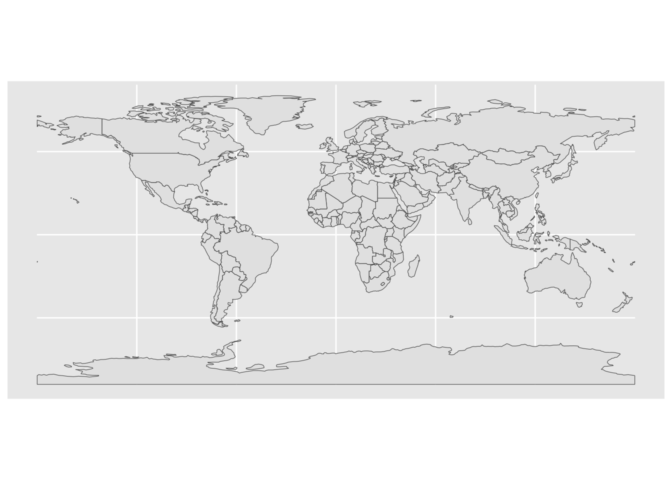

We will begin to get to know the basics of geographic data in R by using the “world” dataset in the package.
First let’s see what information is in the “world” dataset. Get the names of the variables in the world dataset.
Filter the population and GDP data from World map for better understanding the data structure.
Plot the GDP percapita map of the world:
Prepare Africa map by highlighting Zambia

# Select just the continent of Africa
africa <- world %>% 
  filter(region_un %in% "Africa")

Check the type of data

class(africa)

[1] "sf"         "data.frame"

names(africa)

  [1] "featurecla" "scalerank"  "labelrank"  "sovereignt" "sov_a3"    
  [6] "adm0_dif"   "level"      "type"       "tlc"        "admin"     
 [11] "adm0_a3"    "geou_dif"   "geounit"    "gu_a3"      "su_dif"    
 [16] "subunit"    "su_a3"      "brk_diff"   "name"       "name_long" 
 [21] "brk_a3"     "brk_name"   "brk_group"  "abbrev"     "postal"    
 [26] "formal_en"  "formal_fr"  "name_ciawf" "note_adm0"  "note_brk"  
 [31] "name_sort"  "name_alt"   "mapcolor7"  "mapcolor8"  "mapcolor9" 
 [36] "mapcolor13" "pop_est"    "pop_rank"   "pop_year"   "gdp_md"    
 [41] "gdp_year"   "economy"    "income_grp" "fips_10"    "iso_a2"    
 [46] "iso_a2_eh"  "iso_a3"     "iso_a3_eh"  "iso_n3"     "iso_n3_eh" 
 [51] "un_a3"      "wb_a2"      "wb_a3"      "woe_id"     "woe_id_eh" 
 [56] "woe_note"   "adm0_iso"   "adm0_diff"  "adm0_tlc"   "adm0_a3_us"
 [61] "adm0_a3_fr" "adm0_a3_ru" "adm0_a3_es" "adm0_a3_cn" "adm0_a3_tw"
 [66] "adm0_a3_in" "adm0_a3_np" "adm0_a3_pk" "adm0_a3_de" "adm0_a3_gb"
 [71] "adm0_a3_br" "adm0_a3_il" "adm0_a3_ps" "adm0_a3_sa" "adm0_a3_eg"
 [76] "adm0_a3_ma" "adm0_a3_pt" "adm0_a3_ar" "adm0_a3_jp" "adm0_a3_ko"
 [81] "adm0_a3_vn" "adm0_a3_tr" "adm0_a3_id" "adm0_a3_pl" "adm0_a3_gr"
 [86] "adm0_a3_it" "adm0_a3_nl" "adm0_a3_se" "adm0_a3_bd" "adm0_a3_ua"
 [91] "adm0_a3_un" "adm0_a3_wb" "continent"  "region_un"  "subregion" 
 [96] "region_wb"  "name_len"   "long_len"   "abbrev_len" "tiny"      
[101] "homepart"   "min_zoom"   "min_label"  "max_label"  "label_x"   
[106] "label_y"    "ne_id"      "wikidataid" "name_ar"    "name_bn"   
[111] "name_de"    "name_en"    "name_es"    "name_fa"    "name_fr"   
[116] "name_el"    "name_he"    "name_hi"    "name_hu"    "name_id"   
[121] "name_it"    "name_ja"    "name_ko"    "name_nl"    "name_pl"   
[126] "name_pt"    "name_ru"    "name_sv"    "name_tr"    "name_uk"   
[131] "name_ur"    "name_vi"    "name_zh"    "name_zht"   "fclass_iso"
[136] "tlc_diff"   "fclass_tlc" "fclass_us"  "fclass_fr"  "fclass_ru" 
[141] "fclass_es"  "fclass_cn"  "fclass_tw"  "fclass_in"  "fclass_np" 
[146] "fclass_pk"  "fclass_de"  "fclass_gb"  "fclass_br"  "fclass_il" 
[151] "fclass_ps"  "fclass_sa"  "fclass_eg"  "fclass_ma"  "fclass_pt" 
[156] "fclass_ar"  "fclass_jp"  "fclass_ko"  "fclass_vn"  "fclass_tr" 
[161] "fclass_id"  "fclass_pl"  "fclass_gr"  "fclass_it"  "fclass_nl" 
[166] "fclass_se"  "fclass_bd"  "fclass_ua"  "geometry"

Check the data of Africa

africa %>% 
select(sovereignt, gdp_md, gdp_year) %>% 
DT::datatable()

Make professional looking map of Asia

asia <- world[which(world$continent == "Asia"),]
asia.plot = ggplot() +               
  geom_sf(data = asia)  
asia.plot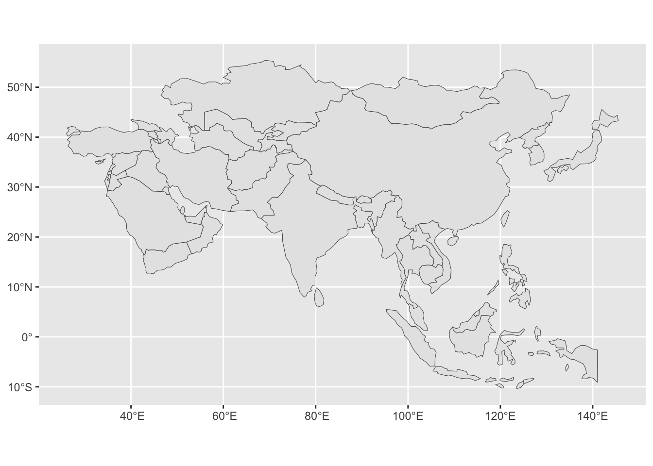

Make professional looking map of Africa

africa <- world[which(world$continent == "Africa"),]
africa.plot = ggplot() +               
  geom_sf(data = africa)  
africa.plot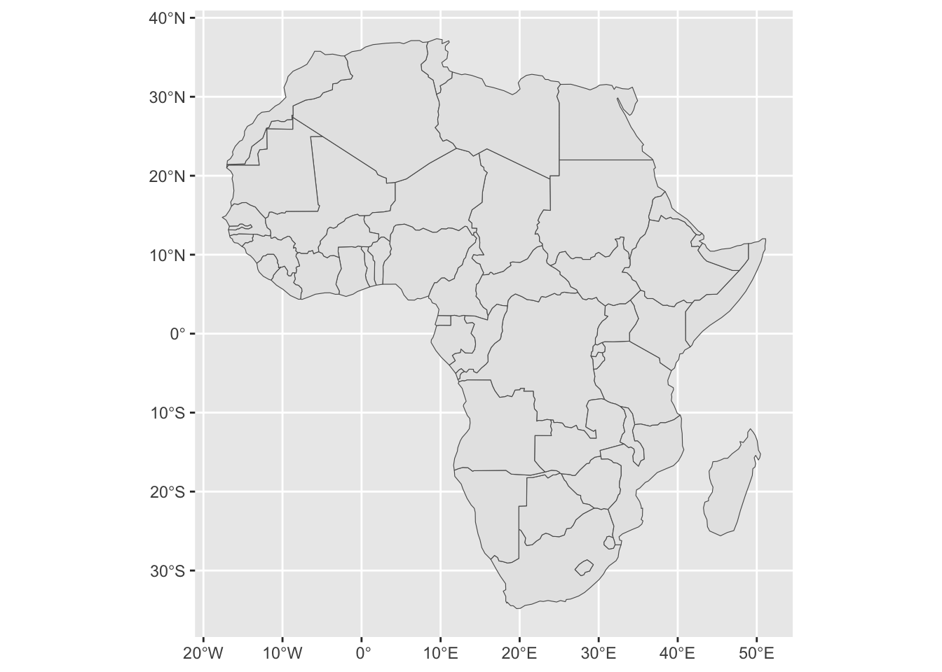

Make professional looking map of Europe

europe <- world[which(world$continent == "Europe"),]
ggplot(europe) +
  geom_sf() +
  coord_sf(xlim = c(-25,50), ylim = c(35,70), expand = FALSE)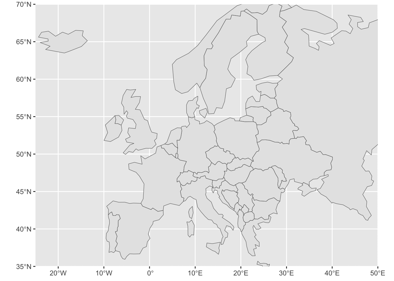

Make professional looking map of Oceania

oceania <- world[which(world$continent == "Oceania"),]
ggplot(oceania) +
  geom_sf() +
  coord_sf(xlim = c(105,180), ylim = c(-50,0), expand = FALSE)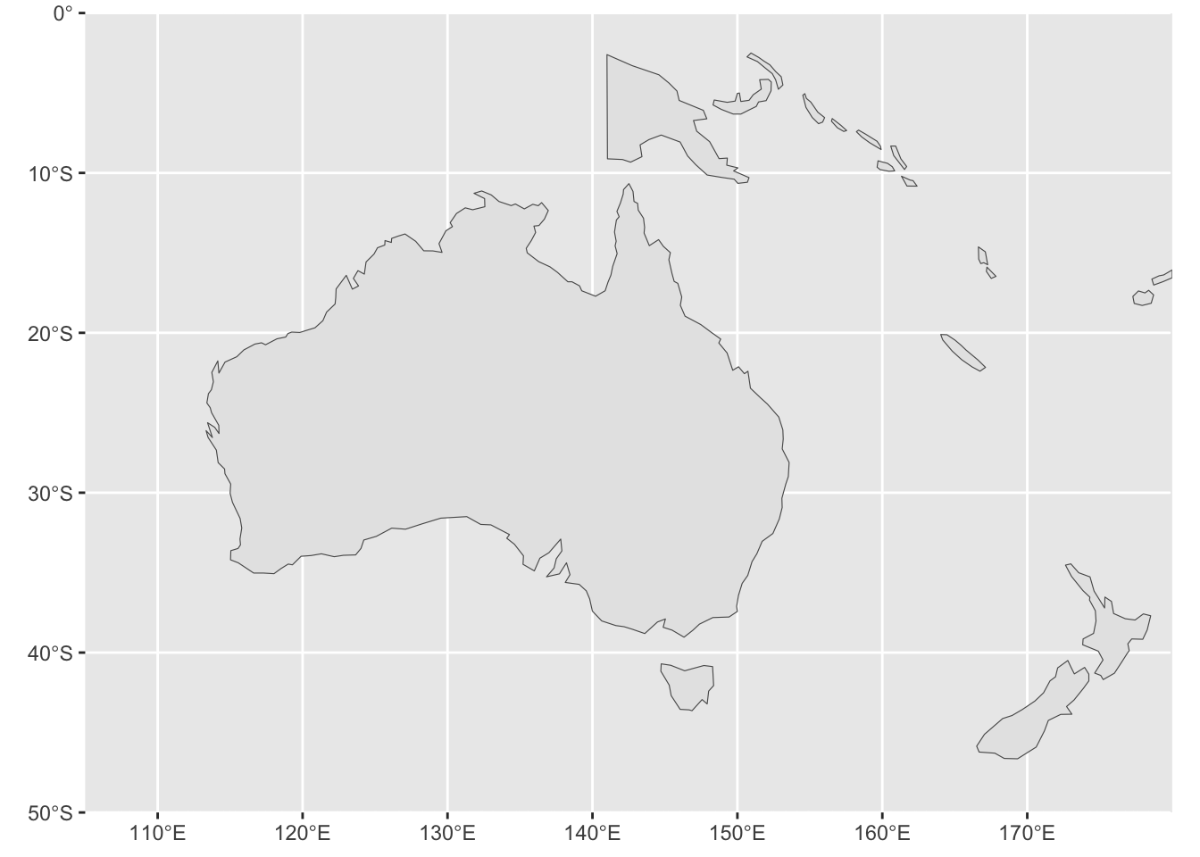

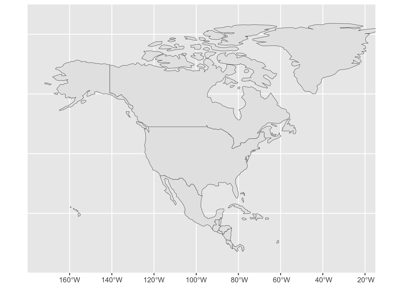
Make professional looking map of North America

north_america <- world[which(world$continent == "North America"),]
ggplot(north_america) +
  geom_sf() +
  coord_sf(xlim = c(-180,-15), ylim = c(0,90), expand = FALSE)

15.1 World and continents with sf

15.1 World and continents with `sf`