pacman::p_load(tidyverse, sf)11 Human geography lab 3
- Load all necessary packages
11.1 Using Shapefile to make map
- Load the
shapefileof Japan’s administrative divisions
jp0_shp <- st_read("data/shapefile/jp_adm0_shp/jpn_admbnda_adm0_2019.shp")
jp1_shp <- st_read("data/shapefile/jp_adm1_shp/jpn_admbnda_adm1_2019.shp")
jp2_shp <- st_read("data/shapefile/jp_adm2_shp/jpn_admbnda_adm2_2019.shp") - Observe the data inside the shape file of
adm0
jp0_shp # for admin level 0
jp1_shp # for admin level 1
jp2_shp # for admin level 2- Check the geographic coordinate system of your
adm0shapefile
st_crs(jp0_shp) # for admin level 0
st_crs(jp1_shp) # for admin level 1
st_crs(jp2_shp) # for admin level 2- Plot the map of Japan admin 0
ggplot(jp0_shp) +
  geom_sf()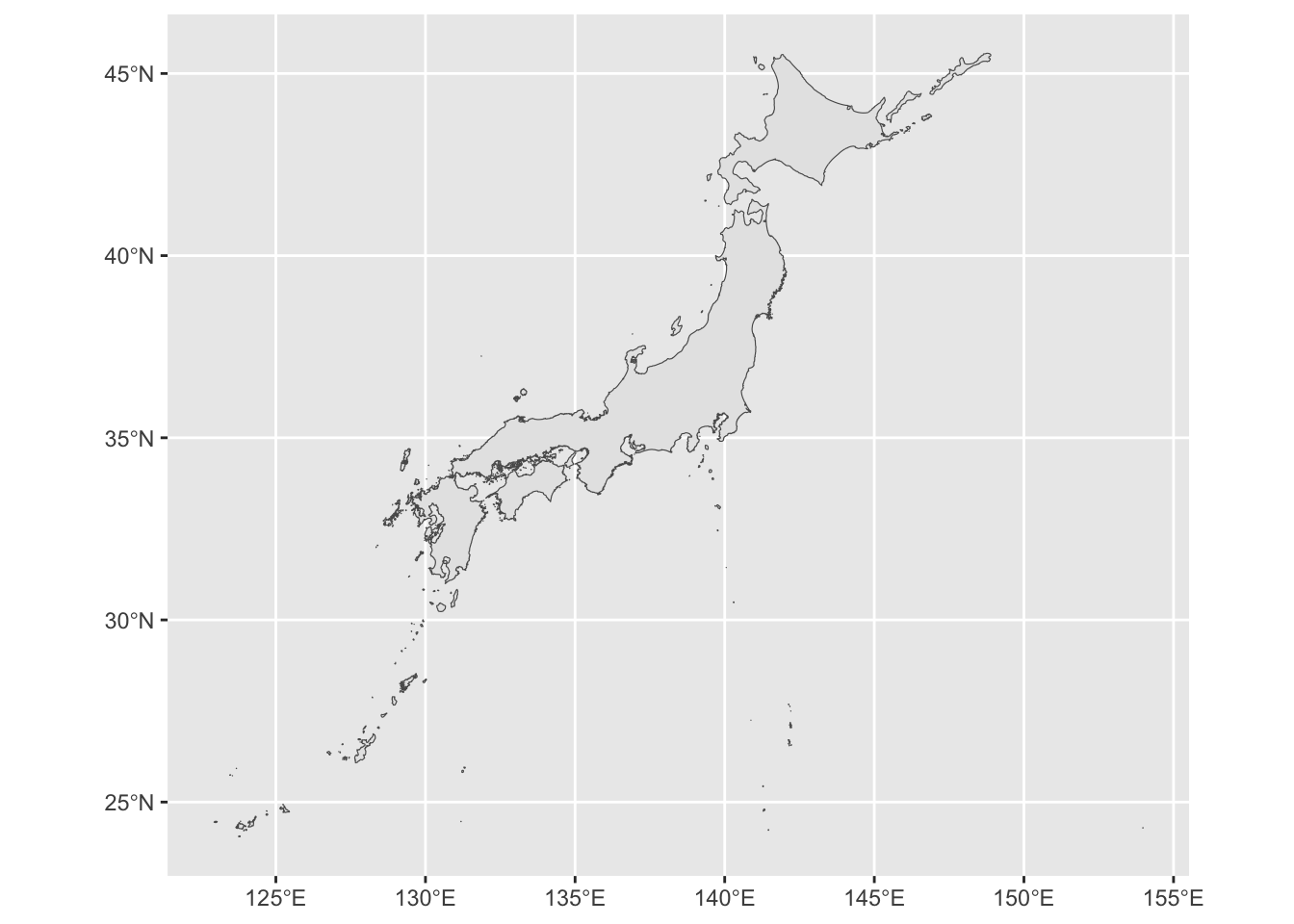
- Change the boundary color and fill it with white color.
ggplot(jp0_shp) +
    geom_sf(color = "blue", fill = "white", lwd = 0.07)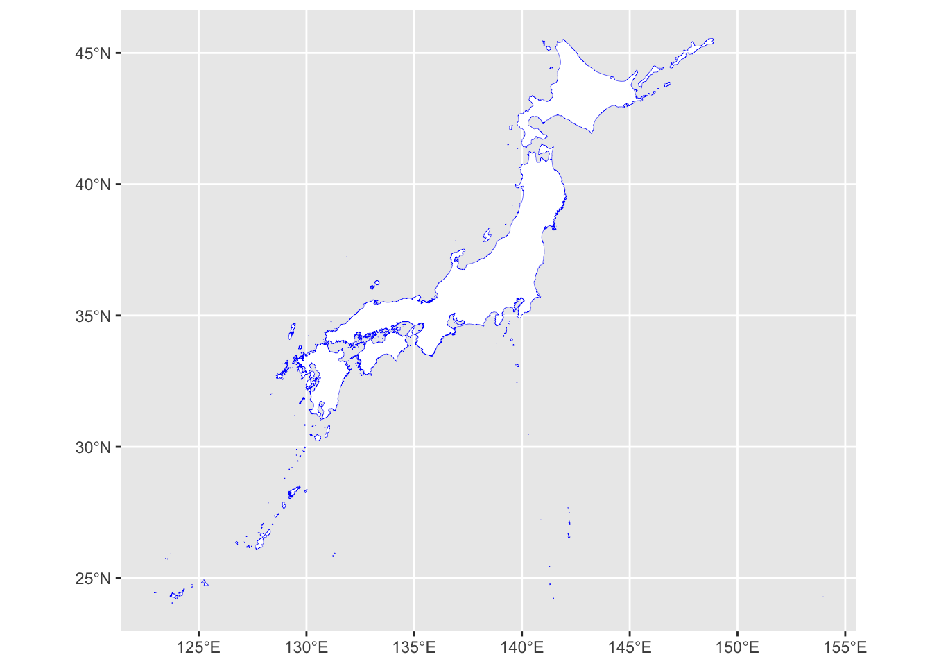
- We can try the
aes()function to improve the visual of the ADM0. Aesthetics are used to bind plotting parameters to your data. Theaes()function defines which variables you want to plot, and which plot parameters to map them to.
ggplot(jp0_shp) +
    geom_sf(aes(fill = ADM0_PCODE),  show.legend = FALSE)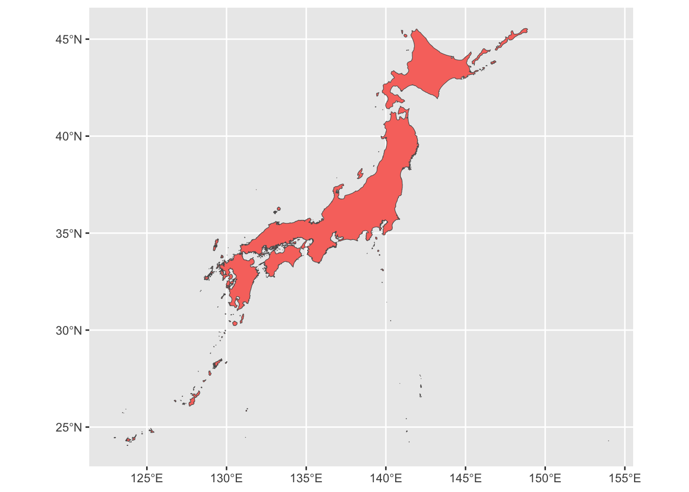
- Plot the map of Japan admin 1
ggplot(jp1_shp) +
  geom_sf()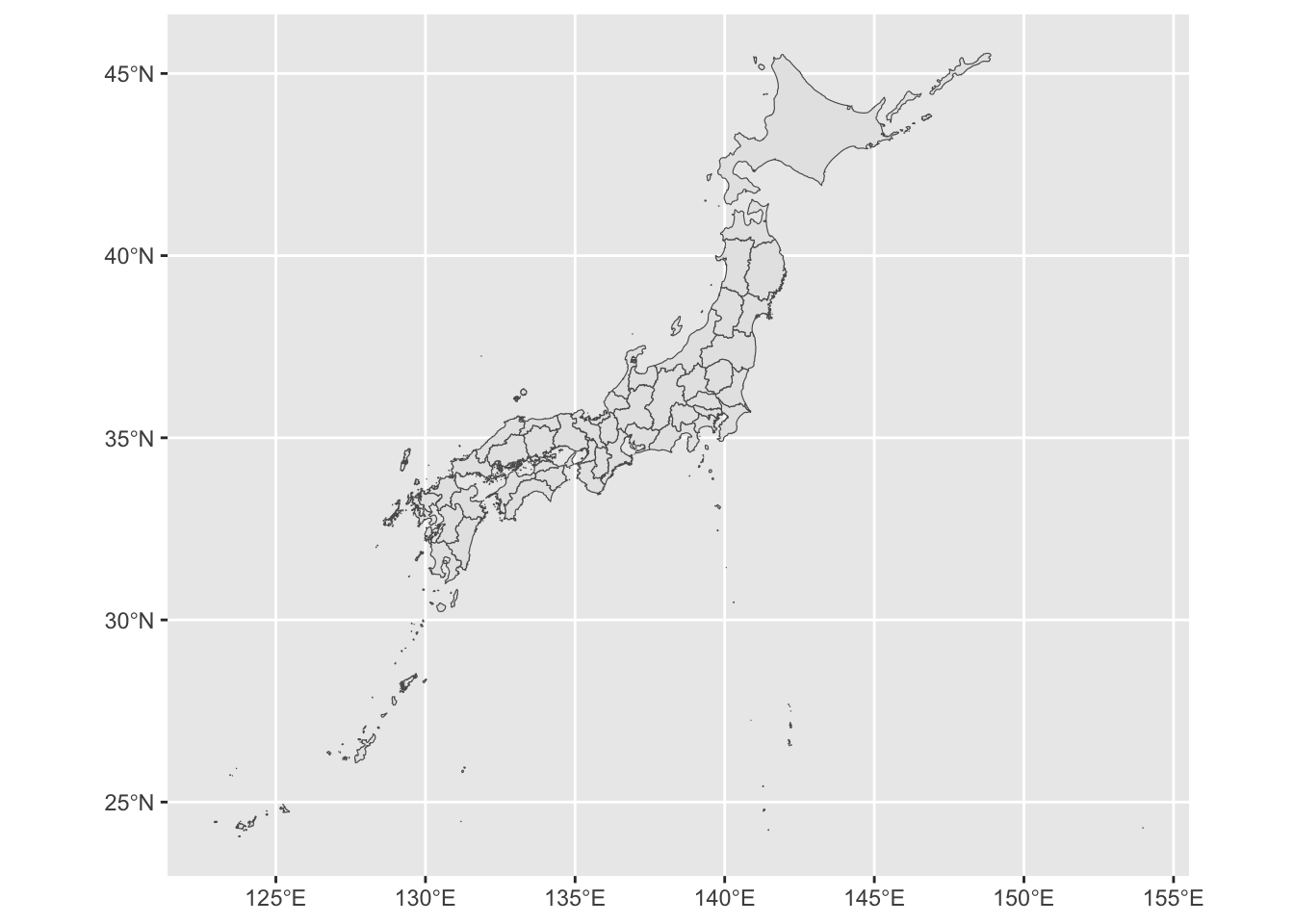
- Lets change the color of boundary and fill.
ggplot(jp1_shp) +
    geom_sf(color = "blue",  fill = "white", lwd = 0.07)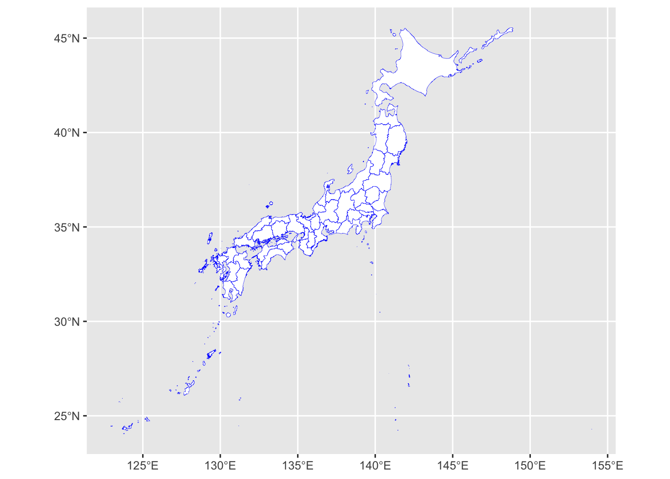
- We can try the
aes()function to improve the visual of the ADM1.
ggplot(jp1_shp) +
    geom_sf(aes(fill = ADM1_PCODE),  show.legend = FALSE)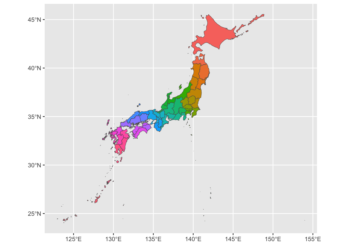
- Plot the map of Japan admin 2
ggplot(jp2_shp) +
  geom_sf()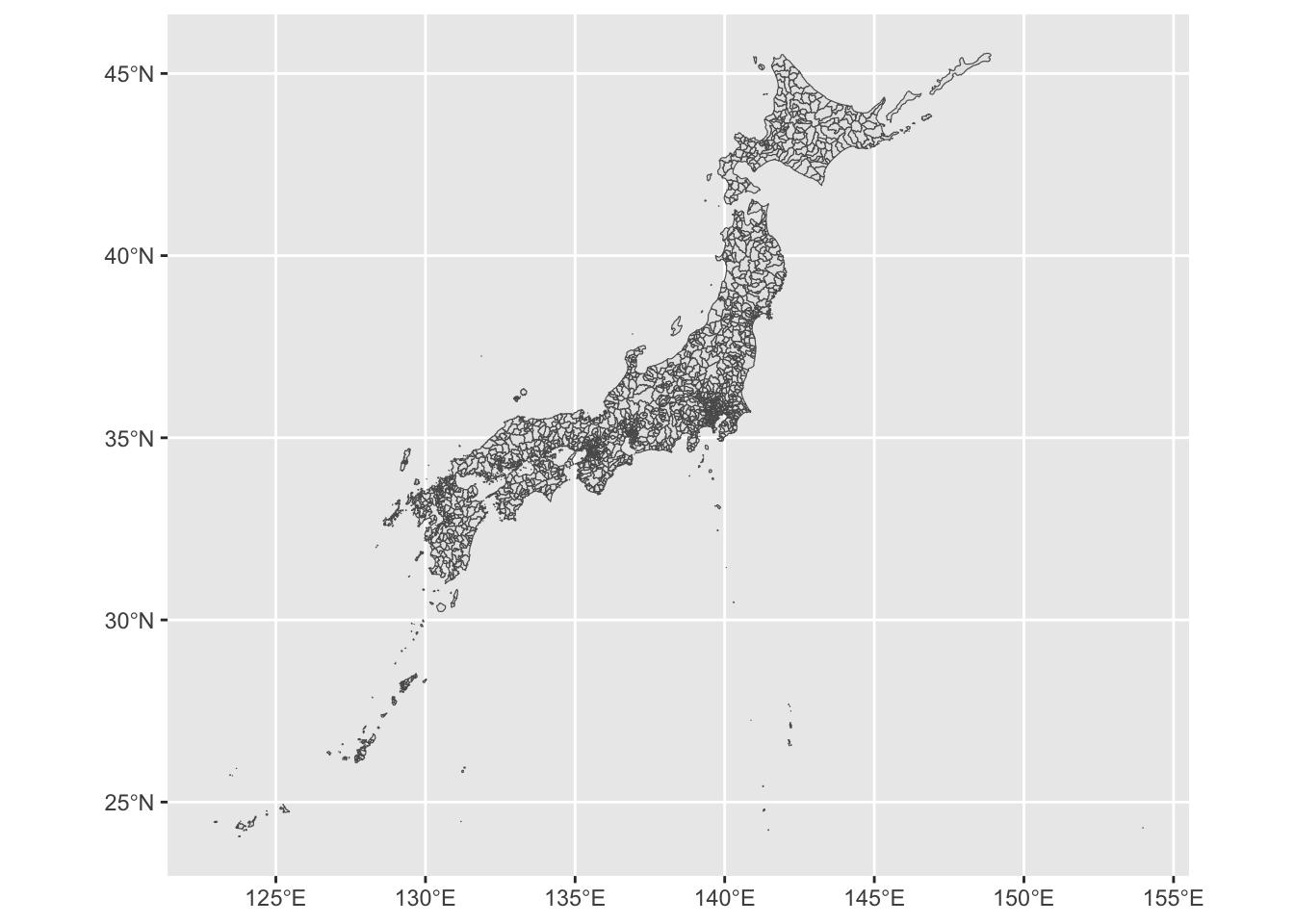
- Lets change the color of boundary and fill
ggplot(jp2_shp) +
    geom_sf(color = "blue",  fill = "white", lwd = 0.07)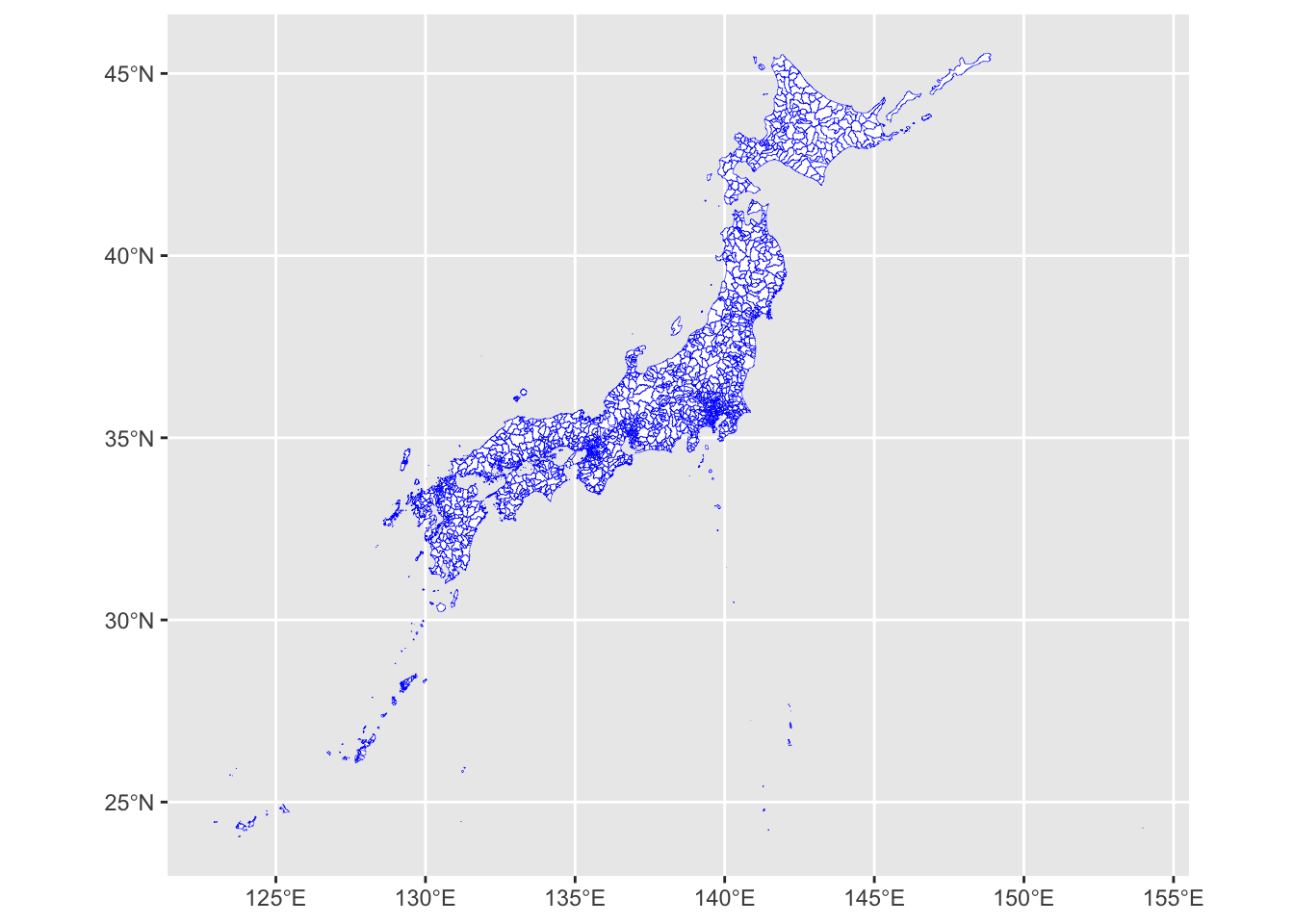
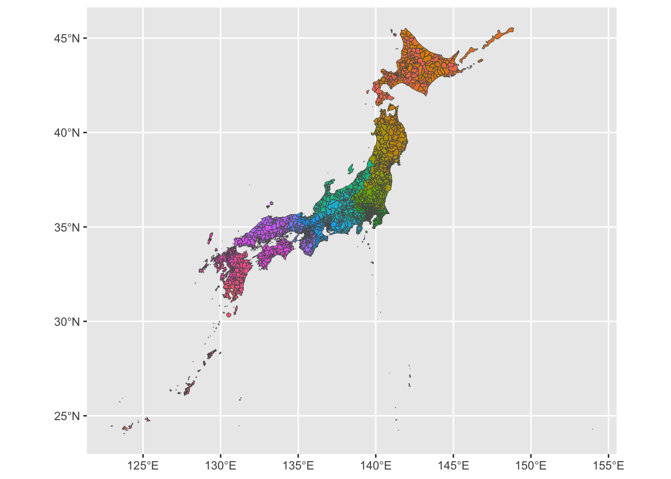
- We can try the
aes()function to improve the visual of the ADM2.
ggplot(jp2_shp) +
    geom_sf(aes(fill = ADM2_PCODE),  show.legend = FALSE)